Computational complexity

Computing integrated information is combinatorially expensive: it searches over subsets, purviews, and partitions of a system, and the number of each grows exponentially or superexponentially with the number of units \(n\). This page has two aims: to give a sense of what each stage costs, and to lay out the options for reducing it by configuring PyPhi to use heuristics. The page focuses on IIT 4.0; actual causation and the earlier IIT 3.0 are covered more briefly at the end.

Formalism	Stage	Dominant cost	Practical ceiling
IIT 4.0	distinctions (CES)	\(\gtrsim 2^n\) mechanisms, super-exponential per pair	~6–8 units
IIT 4.0	relations	up to \(2^{\,2^n-1}-1\)	~6–8 units
IIT 4.0	system \(\varphi_s\)	\(B_n(3)\) directed set partitions	~10–12 units
Actual causation	account	\(2^n\) mechanisms × \(2^n\) purviews × set partitions	~8–10 units
IIT 3.0	CES / subsystem Φ / major complex	\(O(n^5\,3^n)\) / \(6^n\) / \(7^n\)	~10–12 units

The single most expensive term anywhere in IIT is the 4.0 relation count, \(2^{\,2^n-1}-1\) (doubly exponential).

Why it’s expensive: the nested search

Every Φ computation is the same shape of nested loop. Reading from the outside in, the analysis considers:

1. candidate systems — which subset of the substrate is the subject (\(2^n\) subsets);

2. system partitions — cuts that test whether the system is irreducible;

3. mechanisms — subsets of the system that might specify a distinction (\(2^n\));

4. purviews — subsets the mechanism might constrain, on the cause side and the effect side (\(2^n\) each);

5. mechanism partitions — cuts that test whether a mechanism–purview pair is irreducible;

6. sets of distinctions — subsets of the distinctions that might bind into a relation (IIT 4.0 only).

Each level multiplies the work of the levels inside it, and the innermost work — building a repertoire and measuring a distance — is itself polynomial in \(n\). The differences between formalisms are entirely in which levels they visit and how many items each level enumerates, which is set by the configured partition schemes.

The counts at each level are closed-form combinatorial quantities. PyPhi’s enumerators are in pyphi.partition and pyphi.combinatorics.

Quantity	Count	Enumerator
Subsets / mechanisms of \(n\) units	\(2^n\)	pyphi.utils.powerset
Undirected bipartitions	\(2^{\,n-1}\)	pyphi.partition.bipartition()
Directed tripartitions	\(3^n\)	directed_tripartition()
Set partitions	Bell number \(B_n\)	pyphi.combinatorics.set_partitions
Set partitions into \(k\) blocks	Stirling \(S(n,k)\)	k_partitions()
Directed set partitions (4.0 system cuts)	\(\sum_{q\ge 2} S(n,q)\,3^q \sim B_n(3)\)	directed_set_partitions()

The Bell number \(B_n\) already grows faster than any \(c^n\); the “directed” set partitions used for IIT 4.0 system cuts weight each block by one of three directions, giving the Bell polynomial \(B_n(3)\), faster still.

The enumerators below are shown for small n to illustrate the growth. Do not call pyphi.partition.directed_set_partitions() or its relatives directly on ten or more units: they materialize every partition. Use pyphi.cost.estimate_analysis(), which counts without enumerating.

import pandas as pd
from pyphi import combinatorics

def bell(n):
    return sum(1 for _ in combinatorics.set_partitions(range(n)))

pd.DataFrame(
    {
        "n": range(1, 8),
        "subsets 2**n": [2**n for n in range(1, 8)],
        "bipartitions 2**(n-1)": [2 ** (n - 1) for n in range(1, 8)],
        "set partitions B_n": [bell(n) for n in range(1, 8)],
    }
).set_index("n")

	subsets 2**n	bipartitions 2**(n-1)	set partitions B_n
n
1	2	1	1
2	4	2	2
3	8	4	5
4	16	8	15
5	32	16	52
6	64	32	203
7	128	64	877

The inner kernel: one repertoire

The innermost operation builds a repertoire — a probability distribution over the states of a purview — and measures a distance between two of them. A repertoire over a purview of \(p\) units, in a substrate of alphabet size \(k\), is an array of \(k^p\) numbers. PyPhi builds it as a product of per-unit factors over a factored transition-probability matrix (pyphi.core.repertoire_algebra), so a mechanism of \(m\) units costs \(O(m\,k^p)\) multiplications, and the results are memoized so repeated mechanism–purview pairs across the partition sweep are free. IIT 4.0’s intrinsic-difference measures read the distribution in a single pass, \(O(k^p)\). (IIT 3.0 instead uses the earth mover’s distance: \(O(n^2\,3^n)\) in general, or \(O(n)\) for effect repertoires under conditional independence — Mayner et al. 2018.)

The cost of IIT 4.0

IIT 4.0 computes a cause–effect structure — its distinctions and the relations among them — and, at the system level, the system integrated information \(\varphi_s\). These are three separate costs.

Distinctions reuse the mechanism × purview loop: \(2^n - 1\) mechanisms, up to \(2^n - 1\) cause and effect purviews each (pruned by the connectivity matrix), and the mechanism partitions of each pair. The default scheme is JOINT_PARTITION_ALL, which enumerates all set partitions of the mechanism and purview rather than only bipartitions — a Bell-number-weighted count per pair, super-exponential in \(m+p\) and far more than 3.0’s \(2^{\,m+p-1}\). At the sizes actually reachable, the distinctions often dominate the cost, precisely because of this scheme.

Relations are the asymptotically dominant term in all of IIT. A relation binds a set of distinctions that share a congruent purview overlap; over \(n\) units the number of possible relations is doubly exponential (Zaeemzadeh & Tononi, 2024, Sec 2.2):

\[ |R| = 2^{\,2^n - 1} - 1. \]

The counts are computed exactly by pyphi.formalism.iit4.bounds:

import pyphi
from pyphi.formalism.iit4 import bounds

rows = [
    {
        "n": n,
        "possible distinctions (2**n - 1)": bounds.number_of_possible_distinctions(n),
        "possible relations (2**(2**n - 1) - 1)": bounds.number_of_possible_relations(n),
    }
    for n in range(1, 7)
]

import pandas as pd
pd.DataFrame(rows).set_index("n")

	possible distinctions (2**n - 1)	possible relations (2**(2**n - 1) - 1)
n
1	1	1
2	3	7
3	7	127
4	15	32767
5	31	2147483647
6	63	9223372036854775807

By default, relation_computation = "ANALYTICAL" computes the relation count and summed φ in closed form by inclusion–exclusion, without enumerating individual relations at all. Setting relation_computation = "CONCRETE" enumerates them explicitly, but not by walking all \(2^D\) subsets of the \(D\) distinctions found: it walks them depth-first and prunes a whole subtree the moment the running purview overlap becomes empty (pyphi.combinatorics.combinations_with_nonempty_intersection), so the realized count is the number of subsets with nonempty congruent overlap — worst case \(2^D - D - 1\), but typically far fewer. Each candidate relation is lazy: its φ and faces are computed only when read.

System \(\varphi_s\) is separate and much cheaper: it sweeps the DIRECTED_SET_PARTITION system cuts — \(B_n(3)\) before de-duplication — evaluating the whole system at each, with no inner mechanism loop.

The intrinsic-information term of \(\varphi_s\) (Mayner, Marshall & Tononi, 2026, Eq. 23) is evaluated once, at the already-selected minimum-information partition, an \(O(1)\) step that does not change the number of partitions swept; shortcircuit_sia is a constant-factor pre-check that returns early when the system has no cause or effect.

The published φ upper bounds — as opposed to the counts — are also codified, with citations, in pyphi.formalism.iit4.bounds: distinction φ is at most \(|M|\,|Z|\) (Theorem 1), system \(\varphi_s\) at most \(n(n-1)\) (Table 2), the sum of distinction φ grows as \(\approx \tfrac{n^2}{2}2^n\) (Eq. 6), and the sum of relation φ grows hyper-exponentially, \(O(n^2\,2^{\,2^n})\) (Zaeemzadeh & Tononi, 2024). Alongside these worst-case, size-based ceilings, the same module provides measured certificates: given a computed distinction set, sum_phi_relations_measured_bound() evaluates the paper’s linear-program maximum on the measured per-atom profile — a certified bound on the sum of relation φ that is typically orders of magnitude tighter than the worst-case ceiling — and big_phi_measured_bound() adds the exact distinction-φ sum to give a certified ceiling on Φ.

How it scales in practice

benchmarks/complexity/scaling.py times each stage on a family of stochastic-majority ring systems of growing size. Each unit’s next state is a logistic function of the summed spins of its two ring neighbours and itself; the construction is deterministic in \((n, \beta)\), so the systems reproduce exactly. For each size it records several timing trials, saves the raw values, and fits \(\log(\text{time}) = a + b\,n\), whose slope gives the per-unit growth factor \(e^b\).

Note

The timing runs are precomputed, not executed at documentation-build time. Reproduce them with uv run python benchmarks/complexity/scaling.py; the raw timings, aggregates, fitted rates, and figure are written to benchmarks/complexity/results/.

Median wall-clock runtime versus system size \(n\), one curve per stage, on a logarithmic vertical axis. A straight line indicates exponential growth; the upward-bending IIT 4.0 cause–effect-structure curve is super-exponential. IIT 3.0 is shown for comparison.

The IIT 4.0 cause–effect structure grows fastest of all, and not at a fixed base: it is dominated by relations, whose realized count explodes far faster than the number of distinctions.

\(n\)	distinctions	relations
2	3	5
3	7	127
4	15	6 879
5	31	1 413 375

The fitted growth factors (over \(n \ge 3\), where fixed overhead no longer dominates) are below:

Stage	raw base \(e^b\)	base after dividing out \(n^5\)	\(R^2\)
IIT 4.0 — CES	28.1	7.8	0.993
IIT 4.0 — \(\varphi_s\)	7.9	2.8	0.999

Connectivity matters as much as size

The growth factors above are specific to the ring family used for the measurements, and they are best read as a single point in a space parameterized as much by a system’s connectivity as by its size. For a fixed number of units \(n\), the sparsity of the connectivity matrix governs the practical cost through several distinct mechanisms.

The most consequential is purview pruning. A mechanism can constrain only those purviews it reaches through the connectivity matrix, so in a sparsely connected system the number of candidate purviews evaluated per mechanism falls well below \(2^n\). Because the surviving purviews are also smaller, the repertoires and distances computed over them are defined on distributions of correspondingly reduced support (\(k^p\) with \(p \ll n\)); as this per-operation cost enters the exponential base rather than a leading constant, connectivity influences the rate of growth and not merely its scale. Missing connections save work a second way: when they imply that a mechanism’s repertoire factorizes over a purview, the mechanism is reducible over that purview a priori and need not be evaluated at all (Mayner et al., 2018).

Two further reductions act at the system level. A subsystem that is not strongly connected has \(\varphi_s = 0\) by construction and is excluded from the search for the maximal complex, so the measured major-complex cost lies below its \(7^n\) worst case. And because relations are supported on the congruent overlaps of distinction purviews, the smaller and less overlapping purviews of a sparse system yield far fewer realized relations than the \(2^{\,2^n-1}-1\) worst case.

These effects bound the realized cost, not the asymptotic worst case, which is attained at complete connectivity and is unchanged. This qualification matters in practice: integration, the quantity IIT is designed to measure, works against sparsity. The systems of greatest scientific interest tend to be densely connected and therefore costly, while a system sparse enough to fall apart into independent parts has \(\varphi_s = 0\) anyway. Connectivity determines the practical ceiling at least as much as unit count does.

Estimating a workload before running it

Every count above is knowable before any φ is computed. pyphi.estimate_analysis walks the same enumeration machinery the analysis would use — the active system partition scheme, the connectivity-pruned purview sets, the mechanism partitions per (mechanism, purview) size pair — and returns the counts as an AnalysisEstimate, without evaluating anything:

import pyphi
from pyphi import examples

pyphi.estimate_analysis(examples.basic_substrate())

AnalysisEstimate3 units, full

Units	3
State space	8
System partitions	= 22
Specified-state evaluations	16
Mechanisms	7
Purview evaluations	= 30
Mechanism partition sweeps	= 438
Relations	closed form
Possible distinctions	7
Possible relations	127
Capped	False

The estimate reports counts and structural weights (the state-space size is the per-evaluation cost scale); it never predicts wall time, which is machine- and configuration-dependent. It computes no φ, but its counting walk is itself work: on ten fully connected units it takes tens of seconds, and it stops at its limit budget with capped=True, reporting lower bounds; see Estimate the cost before you run for raising the budget. The counterpart for grain searches is SearchBounds.estimate, described in the next section.

The cost of the grain search

The sections above cost a single IIT 4.0 analysis, evaluated at the micro grain. When the units that exist for a substrate are not its smallest parts, the analysis must instead search over grains — grouping micro units into macro units, reading them over windows of several updates, and asking which grouping maximizes \(\varphi_s\) (Marshall et al., 2026). This search wraps a full system-\(\varphi_s\) computation inside a further combinatorial sweep, so its cost is the per-candidate cost of the previous sections multiplied by the number of candidates the sweep visits. The theory is on the macro-units page; running and bounding the search is covered in Search across grains.

The axes of the sweep. Four combinatorial choices compound into the candidate count.

• Decompositions. Partitioning the micro units into groups follows the set-partition growth of the earlier table (Bell numbers), with each group capped at max_constituents units.

• Mappings. Each group of \(|V|\) constituents read over an update grain \(\tau'\) admits \(2^{\,2^{\tau'|V|}} - 2\) non-constant state mappings (Marshall et al., 2026, in the text after Eq. 14). Counted up to complementation of the macro state labels, as PyPhi enumerates them, that is \(2^{\,2^{\tau'|V|} - 1} - 1\), doubly exponential in \(\tau'|V|\): a pair at grain 1 already admits 7, three constituents 127, four constituents 32 767. This is why the default search enumerates only the coarse-graining and blackboxing families and bounds the exhaustive alternative with exhaustive_cap.

• Update grains. Each macroing level contributes its own temporal window, and the grains multiply down a hierarchy of depth max_depth; the product max_update_grain ** max_depth is the length of micro history the search then requires.

• Assemblies. Valid units combine into a candidate system only when their micro footprints and backgrounds are disjoint (Marshall et al., 2026, Eq. 19).

One structural fact keeps this short of the full product of the four axes. The intrinsic-unit criteria (Marshall et al., 2026, Eqs. 16–17) are properties of a decomposition and its background alone — a candidate’s mapping and update grain enter neither inequality — so the search judges each decomposition once, and that single verdict covers all of its variants, whatever their mappings and update grains. Building a unit on meso constituents rather than directly on the micro units narrows the mapping axis further, because the meso units’ own mappings are already fixed (Marshall et al., 2026, Fig. 3E).

What one candidate costs. Each candidate has two separate costs. Constructing its macro transition-probability matrix is \(\Theta(\tau\,4^{n})\) work, whose dominant, mapping-independent share is paid once per distinct (footprint, grain, apportionment) combination rather than once per candidate: those intermediates are cached per substrate (the cache_macro_construction option, on by default), so candidates that differ only in their mapping reuse them. The estimate’s construction_keys_upper_bound counts the distinct (footprint, grain) keys; under the default apportionment="NONE" these are exactly the cached combinations. Evaluating its \(\varphi_s\) is a full IIT 4.0 system analysis over the candidate’s \(m\) macro units, so it sweeps the same DIRECTED_SET_PARTITION system cuts as the previous section, now counted in the macro unit count \(m\):

macro units \(m\)	directed set partitions
1	1
2	3
3	22
4	150
5	1 061
6	7 896

The \(\varphi_s\) evaluations dominate: macro-TPM construction is polynomial in the fixed micro size \(n\), while the partition sweep grows with \(m\) and is paid for every candidate.

Measured shape. On the four-unit substrate of Example 2 from Marshall et al. (2026) — the coarse-graining example worked through in the intrinsic-units tutorial — the default bounds (one macroing level, update grain 1, the coarse-graining and blackboxing families) evaluate about eighty candidate systems and finish in about a second, almost all of it in the \(\varphi_s\) evaluations rather than in constructing the macro TPMs.

Pre-flight before running. Because the candidate count can grow quickly, SearchBounds.estimate counts the systems a set of bounds would visit — walking the search’s own enumerators with lightweight stand-in units — before any macro TPM is built or any \(\varphi_s\) computed:

import numpy as np

from pyphi.macro import SearchBounds
from pyphi.substrate import Substrate

tpm = np.array(
    [
        [0.05, 0.05],
        [0.05, 0.06],
        [0.06, 0.05],
        [0.95, 0.95],
    ]
)
substrate = Substrate(tpm, node_labels=("A", "B"))

estimate = SearchBounds().estimate(substrate)
estimate.distinct_systems_upper_bound

8

The count is an exact worst case: it assumes every judged decomposition passes the criteria, so the search can only do less work than reported, never more. The first-level judgment counts are exact, since the micro units are given, but the mapped and grained variants those judgments spawn already assume every candidate passes, so any macroing level makes the totals a worst case — which is why is_exact is True only at max_depth=0, where no judgment happens at all. The counting walk stops if it exceeds an internal limit (truncated), reporting lower bounds when it does. Comparing distinct_systems_upper_bound against len(result.records) after a run shows how much of the worst case the substrate actually forced.

Reducing the cost

Several options change how much of the search PyPhi actually performs. They fall into three kinds, and the distinction matters for how a result should be read:

• Exact reformulations compute the same answer with less work.

• Approximations trade exactness for speed and return a bound or an estimate.

• Formalism choices change which quantity is computed. Their costs are not comparable as speedups — a different scheme is a different definition, not a faster route to the same number.

Option	Setting	Kind	Effect on cost
relation_computation	ANALYTICAL (default); set CONCRETE to enumerate	exact reformulation (yields the count and summed φ, not individual relations)	removes the \(2^D\) relation enumeration; the CES then scales like its distinctions alone
mechanism_partition_scheme	JOINT_PARTITION_ALL / WEDGE_TRIPARTITION / JOINT_BIPARTITION	formalism choice	per-(mechanism, purview) partition count Bell-weighted \(> 2^{m-1}3^p > 2^{m+p-1}\)
prune (grain search)	"certified" (default); "off" evaluates everything	exact reformulation (identical complexes, ties, and verdicts; skipped candidates report their ii ceiling)	skips candidate partition sweeps certified below an overlapping accepted complex by the requirement; saves most when mapped variants dominate the candidate set; when unit-derivation evaluations dominate, the cost is unchanged
shortcircuit_sia	True	exact early-exit	returns before the sweep when a system has no cause or effect; constant factor
shortcircuit_distinctions	True	exact early-exit	skips a distinction’s remaining search for its maximally irreducible cause and effect (MICE) once one direction is found reducible; on reducible mechanisms this saves an entire purview sweep
parallel	False → True	exact	constant factor set by the number of cores
system_partition_scheme (3.0)	DIRECTED_BIPARTITION → …_CUT_ONE	approximation (upper bound on Φ)	system cuts \(2^n \to 2n\)
assume_partitions_cannot_create_new_concepts (3.0)	False → True	approximation (no guaranteed bound)	reuses the unpartitioned distinctions across cuts

Measured on the same ring family (benchmarks/complexity/options.py):

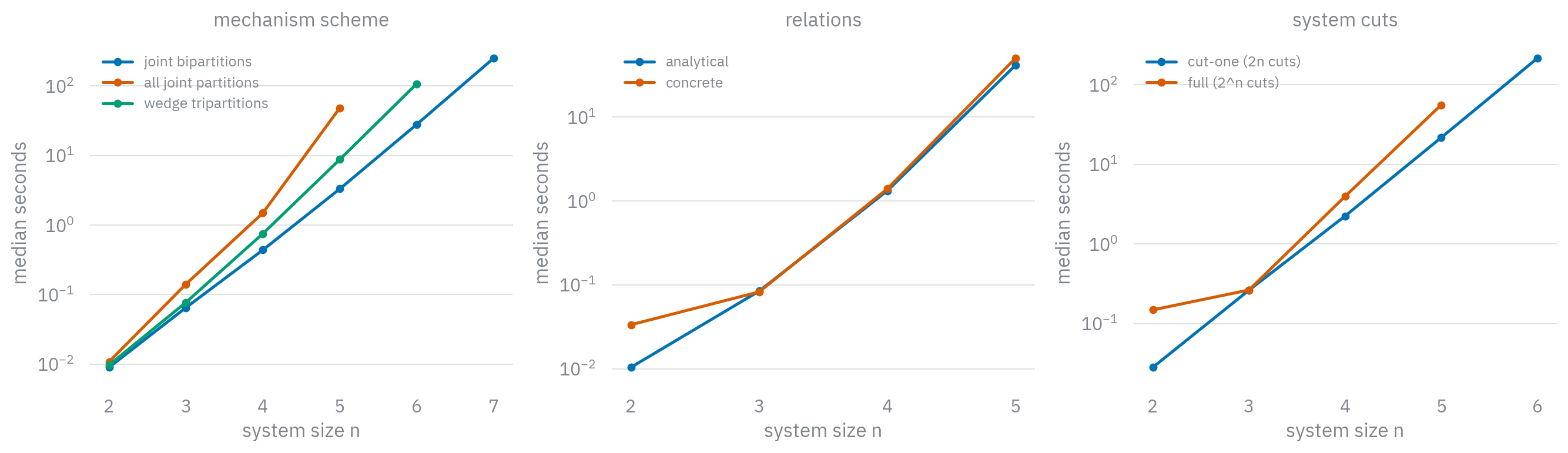
Median runtime versus \(n\) for each option, logarithmic vertical axis. Left: the mechanism partition scheme separates the curves the most — it has the strongest effect on IIT 4.0 distinction cost. Middle: analytical and concrete relations nearly coincide for this system. Right: the IIT 3.0 cut-one approximation is shallower and reaches one unit further than the full cut sweep.

Option	Setting	Median at \(n=5\)	Largest \(n\) under a 45 s/eval budget
mechanism scheme	JOINT_BIPARTITION	3.3 s	7
	WEDGE_TRIPARTITION	8.8 s	6
	JOINT_PARTITION_ALL (default)	48 s	5
relations	ANALYTICAL (default)	41 s	5
	CONCRETE	50 s	5
system cuts (3.0)	cut-one (\(2n\))	22 s	6
	full (\(2^n\), default)	56 s	5

Reading the table, one option at a time:

• The mechanism partition scheme has the largest effect on IIT 4.0 distinction cost. At \(n=5\) the default JOINT_PARTITION_ALL is about 15× slower than JOINT_BIPARTITION, and the gap widens with \(n\): JOINT_BIPARTITION reaches \(n=7\) in ~4 minutes while JOINT_PARTITION_ALL is already at ~48 s by \(n=5\). But this is a formalism choice — the schemes compute different partition families and therefore different φ values, so the cheaper one is a different definition, not a faster route to the same answer.

• Analytical relations help only modestly here, ~1.2× at \(n=5\), because for this system the cause–effect structure cost is dominated by its distinctions, not its relations: the relation term that ANALYTICAL eliminates is not the bottleneck at reachable sizes. Without a per-evaluation time budget, IIT 4.0 CES at \(n=6\) takes about 30 minutes with analytical relations, nearly all of it in the distinctions. On a system with a large, densely overlapping set of distinctions the relation term dominates instead, and the closed form is the difference between tractable and not.

• Cut-one is the most effective approximation for IIT 3.0, ~2.6× at \(n=5\), and it reaches \(n=6\) where the full sweep does not, because it replaces the \(2^n\) system cuts with \(2n\). It returns an upper bound on Φ rather than the exact value.

No single approximation makes IIT 4.0 tractable at larger \(n\): the distinction cost (set by the partition scheme) and the relation cost (set by relation_computation) are separate terms, and reaching higher \(n\) means lowering both.

Stacking settings for working with larger networks

The gains compound. Stacking the compatible cost-reducing settings — rather than any one alone — is what moves the ceiling.

Median runtime versus \(n\) for stacked settings, logarithmic vertical axis. Right, IIT 4.0 CES: bipartitions + analytical (bottom) is far below the others and reaches \(n=7\); the all-partitions + concrete baseline (labeled default in the plot legend) and + analytical coincide. Left, IIT 3.0 big Φ: + cut-one and cut-one + no-new-concepts coincide (lower pair); default and + no-new-concepts coincide (upper pair) — no-new-concepts adds nothing here.

Median seconds, by stack (— = not measured, past the measured size range or the per-evaluation budget):

Stack	\(n=5\)	\(n=6\)	\(n=7\)
IIT 4.0 CES all-partitions + concrete	52	—	—
+ analytical relations	48	—	—
+ bipartitions	13	—	—
bipartitions + analytical	3.3	28	269
IIT 3.0 big Φ default (full cuts)	58	—	—
+ no-new-concepts	61	—	—
+ cut-one	24	225	—
cut-one + no-new-concepts	23	228	—

IIT 4.0 — cheapen distinctions first, then relations. Analytical relations alone barely helps (1.1× at \(n=5\)) because the distinctions dominate. Switching the mechanism scheme to bipartitions cuts the distinction cost ~4×. And once the distinctions are cheap, the relations become the next bottleneck, so analytical relations on top of bipartitions pays off again — another ~4× (\(13 \to 3.3\) s). The two together are ~16× at \(n=5\) and move the ceiling from \(n=5\) to \(n=7\): the full stack reaches seven units (~4.5 min) while all-partitions + concrete is already at ~52 s by five and would take tens of minutes at six. Use this combination when the 4.0 structure needs to be tractable — with the caveat that bipartitions is a formalism choice, so the seven-unit result is a different quantity than the default all-partitions one, not the same number computed faster.

IIT 3.0 — cut-one is the only setting that helps here; no-new-concepts needs a sparse system. Cut-one gives ~2.4× at \(n=5\), growing with \(n\) (the full sweep’s cut count is \(2^n\) against cut-one’s \(2n\)). No-new-concepts, though, gives nothing on this system — it skips re-evaluating mechanisms that do not specify a concept, but this strongly connected ring is dense: every one of the \(2^n-1\) mechanisms specifies a distinction, so there is nothing to skip. No-new-concepts pays off only on sparse systems with few concepts. So cut-one + no-new-concepts is indistinguishable from cut-one alone here.

Neither stack changes the exponential base — they lower the constant and the polynomial factor, buying a unit or two, not a new complexity class. The base is fixed by the formalism.

Practical guidance

• Provide a connectivity matrix. Missing edges let PyPhi prove reducibility without computing repertoires, pruning purviews and cuts a priori.

• For IIT 4.0, cheapen distinctions and relations together. Pairing a cheaper mechanism partition scheme with ANALYTICAL relations compounds — above it reached seven units where all-partitions + concrete stalled at five. The partition scheme is a formalism choice, so this changes which quantity is computed.

• Use ANALYTICAL relations when you need the relation count or summed φ but not the individual relations — it avoids the \(2^D\) enumeration entirely, and helps most once the distinctions are no longer the bottleneck.

• Parallelize (parallel_*_evaluation) and keep repertoire caching on (the default) — the partition sweep revisits the same repertoires many times.

• For IIT 3.0, use cut-one when an upper bound on Φ suffices; its advantage over the full sweep grows with \(n\). No-new-concepts only helps on sparse systems.

IIT 3.0 (historical)

IIT 3.0 has three nested levels, and the exponential base grows at each. One cause–effect structure nests over mechanisms (\(2^n-1\)), cause and effect purviews (up to \(2^n-1\) each, connectivity-pruned), and the JOINT_BIPARTITION mechanism partitions (\(\approx 2^{\,m-1}\cdot 2^p\) per pair). This is \(O(n^5\,3^n)\): the base is \(3\) because each unit is in the mechanism, the purview, or neither — three choices per unit (allowing both would give \(4^n\), which pruning removes), and the \(n^5\) collects the polynomial per-operation work. One subsystem’s Φ recomputes the whole structure for each of the \(2^n\) system cuts, multiplying by \(2^n\) and taking the base to \(6\): \(O(n^5\,6^n)\). The major complex evaluates a subsystem’s Φ for every candidate subsystem; a size-\(k\) subsystem costs \(\sim 6^k\) and there are \(\binom{n}{k}\) of them, so \(\sum_k \binom{n}{k} 6^k = 7^n\) takes the base to \(7\): \(O(n^5\,7^n)\).[1]

The measured growth follows the \(3 \to 6 \to 7\) progression. After dividing out the \(n^5\) polynomial, a single cause–effect structure fits base 3.1 (\(R^2=0.999\)) and one subsystem’s Φ fits 4.7, rising toward 6 at larger sizes. The major complex (Substrate.maximal_complex, timed in benchmarks/complexity/complex_search.py) takes 0.15 / 0.31 / 4.6 / 69 s at \(n = 2/3/4/5\) — at \(n=5\) only ~1.2× the single-subsystem Φ, since the search is dominated by its largest subsystem and the ring prunes non-strongly-connected candidates, holding it below the \(7^n\) worst case.

Two approximations lower the constant: cut-one evaluates only the \(2n\) single-unit cuts rather than all \(2^n\) (an upper bound on Φ), and no-new-concepts reuses the unpartitioned distinctions across cuts (both measured under Reducing the cost, above).

Actual causation

The actual-causation account of a transition nests like a 3.0 cause–effect structure: over the \(2^n-1\) candidate mechanisms, the \(\le 2^n-1\) candidate purviews on each side, and the mechanism partitions (JOINT_PARTITION_ALL, super-exponential per pair), with a full account recomputed for each system cut. Each evaluation compares an actual probability against a partitioned one under the configured α measure (pointwise mutual information, by default). The cost is super-exponential in \(n\), in the same family as the IIT 4.0 distinctions step; the account fits a base of 2.3 after dividing out \(n^5\) over the measured range.

References

• Mayner WGP, Marshall W, Albantakis L, Findlay G, Marchman R, Tononi G (2018). PyPhi: A toolbox for integrated information theory. PLOS Computational Biology 14(7): e1006343.

• Albantakis L, Barbosa L, Findlay G, Grasso M, et al. (2023). Integrated information theory (IIT) 4.0. PLOS Computational Biology 19(10): e1011465.

• Marshall W, Findlay G, Albantakis L, Tononi G (2026). Intrinsic units: identifying a system’s causal grain. Neuroscience of Consciousness 2026(1): niag013.

• Zaeemzadeh A, Tononi G (2024). Upper bounds for integrated information. PLOS Computational Biology 20(8): e1012323.

• Hanson JR, Walker SI (2023). On the non-uniqueness problem in integrated information theory. Neuroscience of Consciousness 2023(1): niad014.

---

[1]

Hanson & Walker (2023) derive \(O(13^m)\) for the major complex by counting “elementary distance calculations”. Their analysis is erroneous because it treats each distance evaluation as a constant-time operation, yet a distance evaluation compares two distributions over the \(2^p\) states of a \(p\)-unit purview and is not constant-time — the general earth mover’s distance is \(O(p^2\,3^p)\) (Mayner et al. 2018), so its cost belongs inside the sum, not as a unit weight. The largest purviews reach \(p \approx m\), so the dominant evaluation alone costs \(O(m^2\,3^m)\); folding this back in raises the base well above 13, so \(O(13^m)\) understates the worst-case operation count by a factor that grows exponentially in \(m\).