Transition probability matrix conventions
A Network can be created with a transition probability matrix (TPM) in any of
the three forms described below. However, in PyPhi the canonical TPM
representation is multidimensional state-by-node form. The TPM will be
converted to this form when the Network is built.
Tip
Functions for converting TPMs from one form to another are available in the
convert module.
State-by-node form
A TPM in state-by-node form is a matrix where the entry \((i,j)\) gives the probability that the \(j^{\textrm{th}}\) node will be ON at time \(t+1\) if the system is in the \(i^{\textrm{th}}\) state at time \(t\).
Multidimensional state-by-node form
A TPM in multidimensional state-by-node form is a state-by-node form that has been reshaped so that it has \(n+1\) dimensions instead of two. The first \(n\) dimensions correspond to each of the \(n\) nodes at time \(t\), while the last dimension corresponds to the probabilities of each node being ON at \(t+1\).
With this form, we can take advantage of NumPy array indexing and use a network state as an index directly:
>>> from pyphi.examples import basic_noisy_selfloop_network
>>> tpm = basic_noisy_selfloop_network().tpm
>>> state = (0, 0, 1)  # A network state is a binary tuple
>>> tpm[state]
array([0.919, 0.91 , 0.756])
This tells us that if the current state is \(N_0 = 0, N_1 = 0, N_2 = 1\), then the for the next state, \(\Pr(N_0 = 1) = 0.919\), \(\Pr(N_1 = 1) = 0.91\) and \(\Pr(N_2 = 1) = 0.756\).
Important
The multidimensional state-by-node form is used throughout PyPhi,
regardless of the form that was used to create the Network.
State-by-state form
A TPM in state-by-state form is a matrix where the entry \((i,j)\) gives the probability that the state at time \(t+1\) will be \(j\) if the state at time \(t\) is labeled by \(i\).
Warning
When converting a state-by-state TPM to one of the other forms, information may be lost!
This is because the space of possible state-by-state TPMs is larger than the space of state-by-node TPMs (so the conversion cannot be injective). However, if we restrict the state-by-state TPMs to only those that satisfy the conditional independence property, then the mapping becomes bijective.
See Conditional Independence for a more detailed discussion.
Little-endian convention
Even after choosing one of the above representations, there are several ways to write down the TPM.
With both state-by-state and state-by-node TPMs, one is confronted with a choice about which rows correspond to which states. In state-by-state TPMs, this choice must also be made for the columns.
There are two possible choices for the rows. Either the first node changes state every other row:
State at \(t\)
\(\Pr(N = ON)\) at \(t+1\)
A, B
A
B
(0, 0)
0.1
0.2
(1, 0)
0.3
0.4
(0, 1)
0.5
0.6
(1, 1)
0.7
0.8
Or the last node does:
State at \(t\)
\(\Pr(N = ON)\) at \(t+1\)
A, B
A
B
(0, 0)
0.1
0.2
(0, 1)
0.5
0.6
(1, 0)
0.3
0.4
(1, 1)
0.7
0.8
Note that the index \(i\) of a row in a TPM encodes a network state: convert the index to binary, and each bit gives the state of a node. The question is, which node?
Throughout PyPhi, we always choose the first convention—the state of the first node (the one with the lowest index) varies the fastest. So, the least-signficant bit—the one’s place—gives the state of the lowest-index node.
This is analogous to the little-endian convention in organizing computer memory. The other convention, where the highest-index node varies the fastest, is analogous to the big-endian convention (see Endianness).
The rationale for this choice of convention is that the little-endian mapping is stable under changes in the number of nodes, in the sense that the same bit always corresponds to the same node index. The big-endian mapping does not have this property.
Tip
Functions to convert states to indices and vice versa, according to either
the little-endian or big-endian convention, are available in the convert
module.
Note
This applies to only situations where decimal indices are encoding states. Whenever a network state is represented as a list or tuple, we use the only sensible convention: the \(i^{\textrm{th}}\) element gives the state of the \(i^{\textrm{th}}\) node.
Connectivity matrix conventions
Throughout PyPhi, if \(CM\) is a connectivity matrix, then \([CM]_{i,j} = 1\) means that there is a directed edge \((i,j)\) from node \(i\) to node \(j\), and \([CM]_{i,j} = 0\) means there is no edge from \(i\) to \(j\).
For example, this network of four nodes
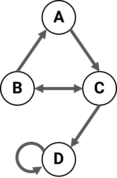
has the following connectivity matrix:
>>> cm = [[0, 0, 1, 0],
...       [1, 0, 1, 0],
...       [0, 1, 0, 1],
...       [0, 0, 0, 1]]